01Advanced Physical Principles & Inverse Lithography Technology (ILT)
Traditional Model-Based OPC operates by fragmenting existing rectangular CAD polygon edges and shifting those segments inward or outward. However, as feature sizes scaled into the sub-3 nm regime under EUV, traditional edge-shifting algorithms hit an absolute mathematical limit in process window optimization.
Inverse Lithography Technology (ILT) treats the mathematical optics transformation as a rigorous, unconstrained inverse mathematical problem. Instead of asking "How should I tweak this rectangle?", ILT solves the wave-equation inverse formulation:
Where:
- \(M\) is the continuous complex mask transmission function.
- \(\text{ForwardOptics}(M)\) models full vector diffraction and resist response.
- \(I_{\text{target}}\) is the desired wafer target layout.
- \(R(M)\) is a regularization term enforcing mask manufacturability constraints.
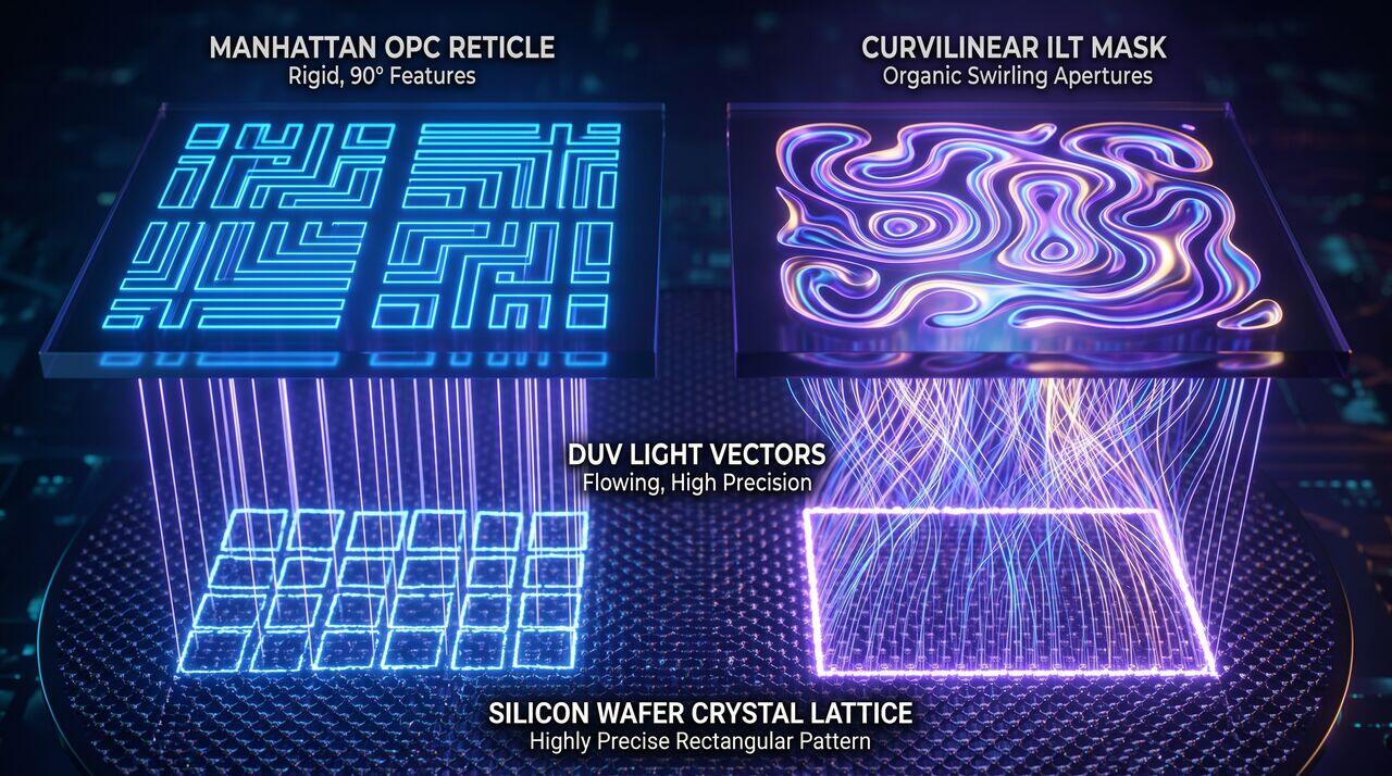
Because ILT solves the inverse wave equation without forcing 90-degree polygon constraints, the resulting mask features are completely curvilinear, featuring organic, highly complex swirling shapes that maximize Normalized Image Log-Slope (NILS) and expand the exposure process window by up to 100%.
02Mathematical Modeling of Photo-Acid Reaction-Diffusion Kinetics
2.1 Coupled Partial Differential Equations for PEB
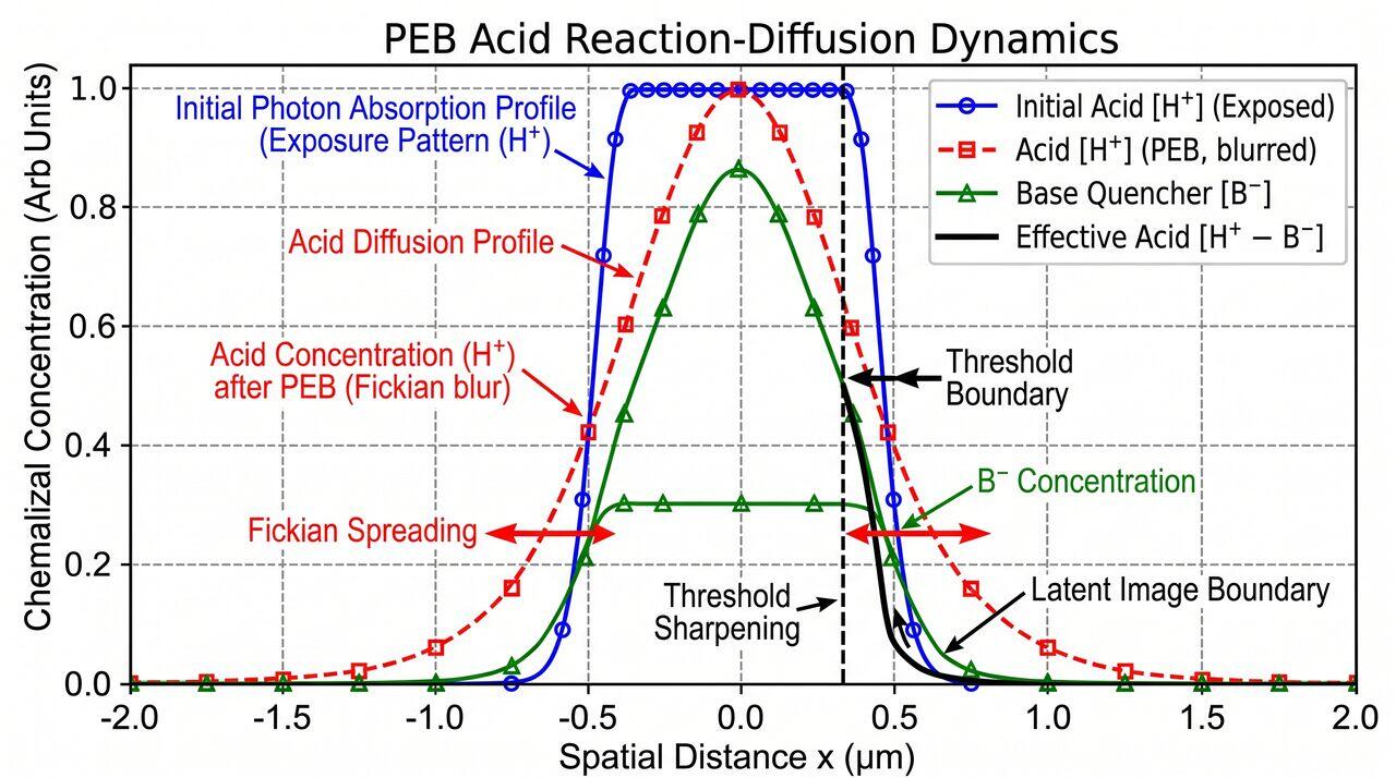
During Post-Exposure Bake (PEB), the spatial and temporal evolution of the photo-acid concentration \([A]\) and the unreacted protective blocking group concentration \([M]\) inside the polymer film is governed by a system of coupled reaction-diffusion partial differential equations:
Where:
- \(D_{\text{acid}}\) is the thermal-dependent Fickian acid diffusion coefficient.
- \(k_{\text{loss}}\) is the neutralization rate constant of photo-acid by added base quencher molecules \([Q]\).
- \(k_{\text{amp}}\) is the catalytic de-protection rate constant.
- \(p\) is the reaction order order parameter.
2.2 Acid Blur vs. Resolution Trade-off
If the acid diffusion coefficient \(D_{\text{acid}}\)\ is too high, the chemical image bleeds across nominal feature boundaries, causing severe acid blur that destroys high-frequency line resolution. Conversely, if \(D_{\text{acid}}\)\ is too low, insufficient chemical amplification occurs, requiring unacceptably high EUV exposure doses. Adding microscopic base quencher molecules (such as photo-decomposable bases, PDB) captures out-diffusing acids at the feature edge, restoring a steep chemical concentration gradient.
03EUV Photon Stochastics & Micro-Bridging Failure Modes
At 13.5 nm EUV wavelength, each individual photon carries an energy of 91.8 eV (compared to 6.4 eV for a 193 nm DUV photon). Consequently, for a given exposure dose (mJ/cm²), an EUV scanner delivers 14 times fewer photons to the photoresist surface than a DUV scanner.
3.1 Poisson Shot Noise Modeling
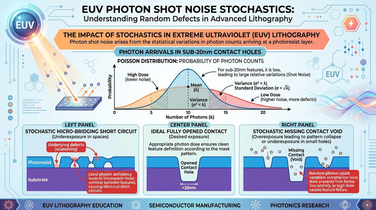
The local arrival of EUV photons in a tiny nanoscale contact hole volume follows a discrete Poisson Distribution:
Where \(\mu\) is the average number of absorbed photons per unit area. At low exposure doses (\(\mu < 50\text{ photons/contact}\)), statistical fluctuations cause some contact holes to absorb insufficient photons, resulting in catastrophic stochastic failures:
- Micro-Bridging: Insufficient photon arrival between adjacent lines leaves un-cleaved polymer behind, creating an electrical short.
- Nano-Porous Voids / Broken Lines: Local statistical lack of acid generation causes complete line interruption (open circuit).
04Media Companion Prompts
Media Prompt 1 (Photorealistic Render)
- Prompt: A striking 3D physics visualization contrasting a traditional 90-degree Manhattan OPC reticle mask with a full Curvilinear Inverse Lithography Technology (ILT) mask. The ILT mask displays smooth, organic fluid-like swirling apertures glowing with deep ultraviolet light vectors, reflecting an ultra-precise rectangular light footprint onto a silicon wafer crystal lattice below. 8k resolution.
Media Prompt 2 (Technical Vector Diagram)
- Prompt: A technical vector plot illustrating acid reaction-diffusion dynamics during Post-Exposure Bake (PEB). Shows chemical concentration profiles vs. spatial distance x: 1) Initial Photon Absorption Profile, 2) Acid Diffusion Profile showing Fickian blur spreading, and 3) Base Quencher Neutralization profile sharpening the chemical threshold boundary.
Media Prompt 3 (Educational Infographic)
- Prompt: An educational infographic detailing EUV Photon Shot Noise stochastics. Displays a Poisson distribution curve of photon arrivals in sub-20nm contact holes. Features sub-panels illustrating microscopic defect mechanisms: Left Panel - Stochastic Micro-Bridging short circuit, Center Panel - Ideal Fully Opened Contact, Right Panel - Stochastic Missing Contact Void.
→Prerequisites & continue reading
Prerequisites: ["p05-t5.3-t2-opc-reticle-enhancement-car-processing-mechanics"]
Also in Topic 5.3, Computational Lithography & OPC:
Tier 1 · OPC, Computational Lithography & Photoresist Fundame…Tier 2 · OPC Reticle Enhancement, Model Calibration & CAR Pro…